Basic Pumping Station
Note
This example focuses on how to implement optimization for pumping stations in RTC-Tools using the Hydraulic Structures library. It assumes basic exposure to RTC-Tools. If you are a first-time user of RTC-Tools, please refer to the RTC-Tools documentation.
The purpose of this example is to understand the technical setup of a model with the Hydraulic Structures Pumping Station object, how to run the model, and how to interpret the results.
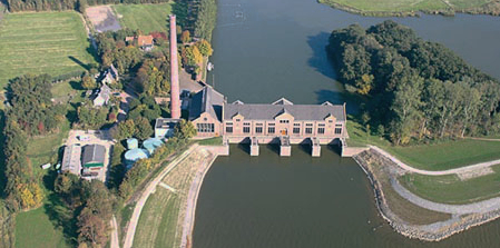
The scenario is the following: A pumping station with a single pump is trying to keep an upstream polder in an allowable water level range. Downstream of the pumping station is a sea with a (large) tidal range, but the sea level never drops below the polder level. Any pump must be on or off for at least a predetermined amount of time. The price on the energy market fluctuates, and the goal of the operator is to keep the polder water level in the allowable range while minimizing the pumping costs.
The folder examples/pumping_station/basic contains the complete RTC-Tools
optimization problem.
The Model
For this example, the model represents a typical setup for a polder pumping station in lowland areas. The inflow from precipitation and seepage is modeled as a discharge (left side), with the total surface area / volume of storage in the polder modeled as a linear storage. The downstream water level is assumed to not be (directly) influenced by the pumping station, and therefore modeled as a boundary condition.
Operating the pumps to discharge the water in the polder consumes power, which varies based on the head difference and total flow. In general, the lower the head difference or discharge, the lower the power needed to pump water.
The expected result is therefore that the model computes a control pattern that makes use of these tidal and energy fluctuations, pumping water when the sea water level is low and/or energy is cheap. It is also expected that as little water as necessary is pumped, i.e. the storage available in the polder is used to its fullest. Concretely speaking this means that the water level at the last time step will be very close (or equal) to the maximum water level.
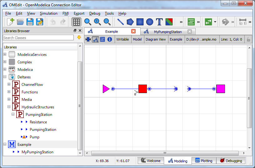
The model can be viewed and edited using the OpenModelica Connection Editor
program. First load the Deltares library into OpenModelica Connection Editor,
and then load the example model, located at
examples/pumping_station/basic/model/Example.mo. The model Example.mo
represents a simple water system with the following elements:
- the polder canals, modeled as storage element
Deltares.ChannelFlow.Hydraulic.Storage.Linear, - a discharge boundary condition
Deltares.ChannelFlow.Hydraulic.BoundaryConditions.Discharge, - a water level boundary condition
Deltares.ChannelFlow.Hydraulic.BoundaryConditions.Level, - a pumping station
MyPumpingStationextendingDeltares.HydraulicStructures.PumpingStation.PumpingStation
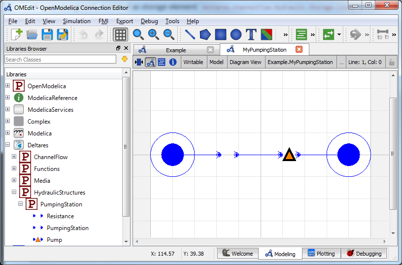
Note it is a nested model. In other words, we have defined our own MyPumpingStation model, which is in itself part of the Example model. You can add classes (e.g. models) to an existing model in the OpenModelica Editor by right clicking your current model (e.g. Example) –> New Modelica Class. Make sure to extend the Deltares.HydraulicStructures.PumpingStation.PumpingStation class.
If we navigate into our nested MyPumpingStation model, we have the following elements:
- our single pump
Deltares.HydraulicStructures.PumpingStation.Pump, - a resistance
Deltares.HydraulicStructures.PumpingStation.Resistance,
In text mode, the Modelica model looks as follows (with annotation statements removed):
1 2 3 4 5 6 7 8 9 10 11 12 13 14 15 16 17 18 19 20 21 22 23 24 25 26 27 28 29 30 31 32 33 34 35 36 37 38 39 40 41 42 43 44 45 46 47 48 49 50 51 52 53 54 55 56 57 58 59 60 61 62 63 64 65 66 67 68 69 70 71 72 73 74 75 76 77 78 79 80 81 82 83 84 85 86 87 88 89 90 91 92 93 94 95 96 97 98 99 100 101 102 103 104 105 106 107 108 109 110 111 112 113 114 115 116 117 118 119 120 121 122 123 124 125 126 127 128 129 130 131 132 133 134 135 136 137 138 139 140 141 142 143 144 145 146 147 148 149 150 151 152 153 154 155 156 157 158 159 160 161 | model Example
model MyPumpingStation
extends Deltares.HydraulicStructures.PumpingStation.PumpingStation(
n_pumps=1
);
Deltares.HydraulicStructures.PumpingStation.Pump pump1(
power_coefficients = {{{-39095.7484857 , 66783.26438029},
{ 7281.58399033, 0.0}},
{{-27859.72396609, 52991.89678362},
{ 6547.78028277, 0.0}},
{{-23247.11759041, 47371.07046571},
{ 6106.48287875, 0.0}},
{{-33451.06236192, 59110.131313 },
{ 7034.0025483, 0.0}},
{{-39861.93265223, 67925.88638803},
{ 7281.81109575, 0.0}},
{{-18905.97159263, 40725.7120928 },
{ 5785.42670305, 0.0}},
{{-69080.26073112, 97844.92974535},
{ 8776.27578528, 0.0}},
{{-27357.47031974, 52938.41395038},
{ 6406.26137405, 0.0}},
{{-49670.43493511, 78653.65042992},
{ 7840.68764271, 0.0}},
{{ -8104.87351317, 21084.47678188},
{ 4586.35220572, 0.0}},
{{-35797.98792283, 54481.08143225},
{ 7595.20055527, 0.0}},
{{-60204.93398172, 89038.39027083},
{ 8408.00958411, 0.0}},
{{-22131.50613895, 39713.73557364},
{ 6465.17137718, 0.0}},
{{-14217.62875014, 34100.99360442},
{ 5201.88819881, 0.0}},
{{-65348.50815507, 94475.38978919},
{ 8575.77174818, 0.0}},
{{-39565.60866869, 63810.57380161},
{ 7597.68369003, 0.0}},
{{-15114.73306987, 33754.82613809},
{ 5508.58396756, 0.0}},
{{-51205.68182194, 79946.23472306},
{ 7963.3995412, 0.0}},
{{ -6701.19277067, 20672.59101587},
{ 4071.93143896, 0.0}},
{{-30637.27553712, 53847.70016923},
{ 6976.92174728, 0.0}},
{{-23174.20780931, 45291.10739497},
{ 6315.4012685, 0.0}},
{{-16838.11645224, 33397.62607586},
{ 5890.34692945, 0.0}},
{{-48684.40184549, 73130.85845968},
{ 8148.05117355, 0.0}},
{{ -5585.5596654 , 17917.6377768 },
{ 3903.50760056, 0.0}},
{{-11530.80023073, 25643.30751799},
{ 5209.61580979, 0.0}},
{{-54050.93126723, 81474.03659672},
{ 8244.19508265, 0.0}},
{{-17059.63308541, 38705.96069607},
{ 5468.15043893, 0.0}},
{{-42990.53693314, 61384.80799185},
{ 8077.30306983, 0.0}},
{{-28740.24310978, 47105.49859182},
{ 7058.4428374, 0.0}},
{{ -9433.46984887, 26148.5409928 },
{ 4488.53180172, 0.0}},
{{-54478.410763 , 83635.76502236},
{ 8076.34522102, 0.0}},
{{-34733.3023365 , 61966.5148778 },
{ 6963.68444901, 0.0}},
{{ -4371.73397616, 13785.26261371},
{ 3759.68617973, 0.0}},
{{-44469.5263585 , 71683.6367841 },
{ 7713.90758475, 0.0}},
{{-10835.36867811, 27900.70743971},
{ 4844.53856386, 0.0}}},
working_area = {{{ -5.326999, 54.050758},
{ -1.0, 0.0}},
{{-0.75242261, 2.79784166},
{-1.0, 0.0}},
{{-0.50567904, 2.3278547},
{-1.0, 0.0}},
{{-1.31944138, 3.6515112},
{-1.0, 0.0}},
{{-1.93409137, 4.35798345},
{-1.0, 0.0}},
{{-1.04947144, 3.27458583},
{-1.0, 0.0}},
{{ 2.577975, -5.203480},
{-1.0, 0.0}},
{{18.23055367, -15.4218745},
{-1.0, 0.0}},
{{16.79364838, -13.50826804},
{-1.0, 0.0}},
{{14.2340237, -8.67903153},
{-1.0, 0.0}},
{{19.76140152, -17.16334892},
{-1.0, 0.0}},
{{15.40792185, -11.24444311},
{-1.0, 0.0}}},
speed_coefficients = {{88.3224, 281.642, 143.011},
{58.8183, -24.9845, 0.0},
{-1.45483, 0.0, 0.0}},
working_area_direction = {1, -1, -1, -1, -1, -1, -1, 1, 1, 1, 1, 1},
minimum_on=3.0*3600
);
Deltares.HydraulicStructures.PumpingStation.Resistance resistance1(C=0.0);
equation
connect(HQUp, resistance1.HQUp);
connect(resistance1.HQDown, pump1.HQUp);
connect(pump1.HQDown, HQDown);
end MyPumpingStation;
// Elements in model flow chart
Deltares.ChannelFlow.Hydraulic.Storage.Linear storage(
A = 149000,
H_b = -1.0,
HQ.H(min = -0.7, max = 0.2),
V(nominal = 1E5)
);
Deltares.ChannelFlow.Hydraulic.BoundaryConditions.Level sea;
Deltares.ChannelFlow.Hydraulic.BoundaryConditions.Discharge inflow;
MyPumpingStation pumpingstation1;
// Input variables
input Modelica.SIunits.VolumeFlowRate Q_in(fixed = true);
input Modelica.SIunits.Position H_ext(fixed=true);
// Energy price is typically of units EUR/kWh (when optimizing for energy
// usage), but one can also choose for e.g. ton CO2/kWh to get the lowest
// CO2 output.
input Real energy_price(fixed=true);
// NOTE: Because we cannot flag each pump's .Q as "input", we need an extra
// variable to do this. Format is expected to be the fully specified name,
// with all dots replaced with underscores.
input Real pumpingstation1_pump1_Q;
// TODO: Move bounds to the mixin.
input Real pumpingstation1_resistance1_dH(min=0.0, max=10.0);
// Output variables
output Modelica.SIunits.Position storage_level;
output Modelica.SIunits.Position sea_level;
equation
connect(pumpingstation1.HQUp, storage.HQ);
connect(pumpingstation1.HQDown, sea.HQ);
connect(inflow.HQ, storage.HQ);
// Mapping of variables
inflow.Q = Q_in;
sea.H = H_ext;
pumpingstation1.pump1.Q = pumpingstation1_pump1_Q;
pumpingstation1.resistance1.dH = pumpingstation1_resistance1_dH;
storage_level = storage.HQ.H;
sea_level = H_ext;
end Example;
|
The attributes of pump1 are explained in detail in Pump.
In addition to the elements, two input variables pumpingstation1_pump1_Q
and pumpingstation1_resistance1_dH are also defined, with a set of
equations matching them to their dot-equivalent (e.g.
pumpingstation1.pump1.Q).
Important
Because nested input symbols cannot be detected, it is necessary for the
user to manually map this symbol to an equivalent one with dots replaced
with underscores.
The Optimization Problem
The python script consists of the following blocks:
- Import of packages
- Definition of water level goal
- Definition of the optimization problem class
- Constructor
- Passing a list of pumping stations
- Additional configuration of the solver
- A run statement
Importing Packages
For this example, the import block is as follows:
1 2 3 4 5 6 7 8 9 10 | import os
from datetime import timedelta
from rtctools.optimization.collocated_integrated_optimization_problem import CollocatedIntegratedOptimizationProblem
from rtctools.optimization.goal_programming_mixin import GoalProgrammingMixin, StateGoal
from rtctools.optimization.linearized_order_goal_programming_mixin import LinearizedOrderGoalProgrammingMixin
from rtctools.optimization.modelica_mixin import ModelicaMixin
from rtctools.optimization.pi_mixin import PIMixin
from rtctools.util import run_optimization_problem
|
Note that we are importing both PumpingStationMixin and PumpingStation
from rtctools_hydraulic_structures.pumping_station_mixin.
Water Level Goal
Next we define our water level range goal. It reads the desired upper and
lower water levels from the optimization problem class. For more information
about how this goal maps to an objective and constraints, we refer to the
documentation of
StateGoal.
15 16 17 18 19 20 21 22 23 24 25 26 27 28 29 30 31 32 | class WaterLevelRangeGoal(StateGoal):
"""
Goal that tries to keep the water level minum and maximum water level,
the values of which are read from the optimization problem.
"""
state = 'storage.HQ.H'
priority = 1
def __init__(self, optimization_problem):
self.target_min = optimization_problem.wl_min
self.target_max = optimization_problem.wl_max
_range = self.target_max - self.target_min
self.function_range = (self.target_min - _range, self.target_max + _range)
super().__init__(optimization_problem)
|
Optimization Problem
Then we construct the optimization problem class by declaring it and inheriting the desired parent classes.
35 36 37 | class Example(PumpingStationMixin,
LinearizedOrderGoalProgrammingMixin, GoalProgrammingMixin,
PIMixin, ModelicaMixin, CollocatedIntegratedOptimizationProblem):
|
Now we define our pumping station objects, and store them in a local instance
variable. We refer to this instance variable from the abstract method
pumping_stations() we have to override.
51 52 53 54 55 56 57 |
# Here we define a list of pumping stations, each consisting of a list
# of pumps. In our case, there is only one pumping station containing
# a single pump.
self.__pumping_stations = [PumpingStation(self, 'pumpingstation1',
pump_symbols=['pumpingstation1.pump1'],
energy_price_symbols='energy_price')]
|
59 60 61 62 63 | def pumping_stations(self):
# This is the method that we must implement. It has to return a list of
# PumpingStation objects, which we already initialized in the __init__
# function. So here we just return that list.
return self.__pumping_stations
|
Then we append our water level range goal to the list of path goals from our parents classes:
70 71 72 73 | def path_goals(self):
goals = super().path_goals()
goals.append(WaterLevelRangeGoal(self))
return goals
|
We also add a minimization goal for the costs, which has a default priority of
sys.maxsize. This goal will automatically integrate the product of power
and energy price for all pumps in all pumping stations,
65 66 67 68 | def goals(self):
goals = super().goals()
goals.append(MinimizePumpCostGoal(self))
return goals
|
Finally, we want to apply some additional configuration, reducing the amount of information the solver outputs:
75 76 77 78 79 | def solver_options(self):
options = super().solver_options()
options['solver'] = 'cbc'
options['casadi_solver'] = 'qpsol'
return options
|
Run the Optimization Problem
To make our script run, at the bottom of our file we just have to call
the run_optimization_problem() method we imported on the optimization
problem class we just created.
184 | run_optimization_problem(Example, base_folder='..')
|
The Whole Script
All together, the whole example script is as follows:
1 2 3 4 5 6 7 8 9 10 11 12 13 14 15 16 17 18 19 20 21 22 23 24 25 26 27 28 29 30 31 32 33 34 35 36 37 38 39 40 41 42 43 44 45 46 47 48 49 50 51 52 53 54 55 56 57 58 59 60 61 62 63 64 65 66 67 68 69 70 71 72 73 74 75 76 77 78 79 80 81 82 83 84 85 86 87 88 89 90 91 92 93 94 95 96 97 98 99 100 101 102 103 104 105 106 107 108 109 110 111 112 113 114 115 116 117 118 119 120 121 122 123 124 125 126 127 128 129 130 131 132 133 134 135 136 137 138 139 140 141 142 143 144 145 146 147 148 149 150 151 152 153 154 155 156 157 158 159 160 161 162 163 164 165 166 167 168 169 170 171 172 173 174 175 176 177 178 179 180 181 182 183 184 | import os
from datetime import timedelta
from rtctools.optimization.collocated_integrated_optimization_problem import CollocatedIntegratedOptimizationProblem
from rtctools.optimization.goal_programming_mixin import GoalProgrammingMixin, StateGoal
from rtctools.optimization.linearized_order_goal_programming_mixin import LinearizedOrderGoalProgrammingMixin
from rtctools.optimization.modelica_mixin import ModelicaMixin
from rtctools.optimization.pi_mixin import PIMixin
from rtctools.util import run_optimization_problem
from rtctools_hydraulic_structures.pumping_station_mixin import \
MinimizePumpCostGoal, PumpingStation, PumpingStationMixin, plot_operating_points
class WaterLevelRangeGoal(StateGoal):
    """
    Goal that tries to keep the water level minum and maximum water level,
    the values of which are read from the optimization problem.
    """

    state = 'storage.HQ.H'

    priority = 1

    def __init__(self, optimization_problem):
        self.target_min = optimization_problem.wl_min
        self.target_max = optimization_problem.wl_max

        _range = self.target_max - self.target_min
        self.function_range = (self.target_min - _range, self.target_max + _range)

        super().__init__(optimization_problem)
class Example(PumpingStationMixin,
              LinearizedOrderGoalProgrammingMixin, GoalProgrammingMixin,
              PIMixin, ModelicaMixin, CollocatedIntegratedOptimizationProblem):
"""
An example showing the basic usage of the PumpingStationMixin. It consists of two goals:
1. Keep water level in the acceptable range.
2. Minimize power usage for doing so.
"""
# Set the target minimum and maximum water levels.
wl_min, wl_max = (-0.5, 0)
def __init__(self, *args, **kwargs):
super().__init__(*args, **kwargs)
self.__output_folder = kwargs['output_folder'] # So we can write our pictures to it
        # Here we define a list of pumping stations, each consisting of a list
        # of pumps. In our case, there is only one pumping station containing
        # a single pump.
        self.__pumping_stations = [PumpingStation(self, 'pumpingstation1',
                                                  pump_symbols=['pumpingstation1.pump1'],
                                                  energy_price_symbols='energy_price')]
    def pumping_stations(self):
        # This is the method that we must implement. It has to return a list of
        # PumpingStation objects, which we already initialized in the __init__
        # function. So here we just return that list.
        return self.__pumping_stations
def goals(self):
goals = super().goals()
goals.append(MinimizePumpCostGoal(self))
return goals
    def path_goals(self):
        goals = super().path_goals()
        goals.append(WaterLevelRangeGoal(self))
        return goals
    def solver_options(self):
        options = super().solver_options()
        options['solver'] = 'cbc'
        options['casadi_solver'] = 'qpsol'
        return options
def post(self):
super().post()
results = self.extract_results()
# TODO: Currently we use hardcoded references to pump1. It would be
# prettier if we could generalize this so we can handle an arbitrary
# number of pumps. It would also be prettier to replace hardcoded
# references to e.g. pumpingstation1.pump1__power with something like
# pumpingstation1.pump.power(), if at all possible.
# Calculate the total amount of energy used. Note that QHP fit was
# made to power in W, and that our timestep is 1 hour.
powers = results['pumpingstation1.pump1__power'][1:]
total_power = sum(powers)/1000
print("Total power = {} kWh".format(total_power))
# Calculate total energy cost
price = self.get_timeseries('energy_price').values[1:]
cost = sum(powers*price)/1000
print("Total cost = {} Euro".format(cost))
# Make plots
import matplotlib.dates as mdates
import matplotlib.pyplot as plt
import numpy as np
plt.style.use('ggplot')
def unite_legends(axes):
handles, labels = [], []
for ax in axes:
tmp = ax.get_legend_handles_labels()
handles.extend(tmp[0])
labels.extend(tmp[1])
return handles, labels
# Discard history from plotting.
i_start = list(self.get_timeseries('energy_price', 0).times).index(self.initial_time)
# Plot #1: Data over time. X-axis is always time.
f, axarr = plt.subplots(5, sharex=True)
times = [self.io.reference_datetime + timedelta(seconds=s) for s in self.times()]
axarr[0].set_ylabel('Water level\n[m]')
axarr[0].plot(times, results['storage_level'], label='Polder',
linewidth=2, color='b')
axarr[0].plot(times, self.wl_max * np.ones_like(times), label='Polder Max',
linewidth=2, color='r', linestyle='--')
axarr[0].plot(times, self.wl_min * np.ones_like(times), label='Polder Min',
linewidth=2, color='g', linestyle='--')
ymin, ymax = axarr[0].get_ylim()
axarr[0].set_ylim(ymin - 0.1, ymax + 0.1)
axarr[1].set_ylabel('Water level\n[m]')
axarr[1].plot(times, self.get_timeseries('H_ext', 0).values[i_start:], label='Sea',
linewidth=2, color='b')
ymin, ymax = axarr[1].get_ylim()
axarr[1].set_ylim(ymin - 0.5, ymax + 0.5)
axarr[2].set_ylabel('Energy price\n[EUR/kWh]')
axarr[2].step(times, self.get_timeseries('energy_price', 0).values[i_start:], label='Energy price',
linewidth=2, color='b')
ymin, ymax = axarr[2].get_ylim()
axarr[2].set_ylim(-0.1, ymax + 0.1)
axarr[3].set_ylabel('Discharge\n[$\\mathdefault{m^3\\!/s}$]')
axarr[3].step(times, results['pumpingstation1.pump1.Q'], label='Pump',
linewidth=2, color='b')
axarr[3].plot(times, self.get_timeseries('Q_in', 0).values[i_start:], label='Inflow',
linewidth=2, color='g')
ymin, ymax = axarr[3].get_ylim()
axarr[3].set_ylim(-0.05 * (ymax - ymin), ymax * 1.1)
axarr[3].xaxis.set_major_formatter(mdates.DateFormatter('%H:%M'))
axarr[4].set_ylabel('Pump speed\n[$\\mathdefault{min^{-1}}$]')
axarr[4].step(times, results['pumpingstation1.pump1_speed'], label='Speed',
linewidth=2, color='b')
ymin, ymax = axarr[4].get_ylim()
axarr[4].set_ylim(-0.05 * (ymax - ymin), ymax * 1.1)
axarr[4].xaxis.set_major_formatter(mdates.DateFormatter('%H:%M'))
for ax in axarr:
ax.set_xlim(min(times), max(times))
f.autofmt_xdate()
# Shrink each axis by 20% and put a legend to the right of the axis
for i in range(len(axarr)):
box = axarr[i].get_position()
axarr[i].set_position([box.x0, box.y0, box.width * 0.8, box.height])
axarr[i].legend(loc='center left', bbox_to_anchor=(1, 0.5), frameon=False)
# Output Plot
f.set_size_inches(8, 9)
plt.savefig(os.path.join(self.__output_folder, 'overall_results.png'), bbox_inches='tight', pad_inches=0.1)
# Plot the working area with the operating points of the pump.
plot_operating_points(self, self.__output_folder)
# Run
run_optimization_problem(Example, base_folder='..')
|
Results
The results from the run are found in output/timeseries_export.xml. Any
PI-XML-reading software can import it.
The post() method in our Example class also generates some pictures to
help understand what is going on.
First we have an overview of the relevant boundary conditions and control variables.
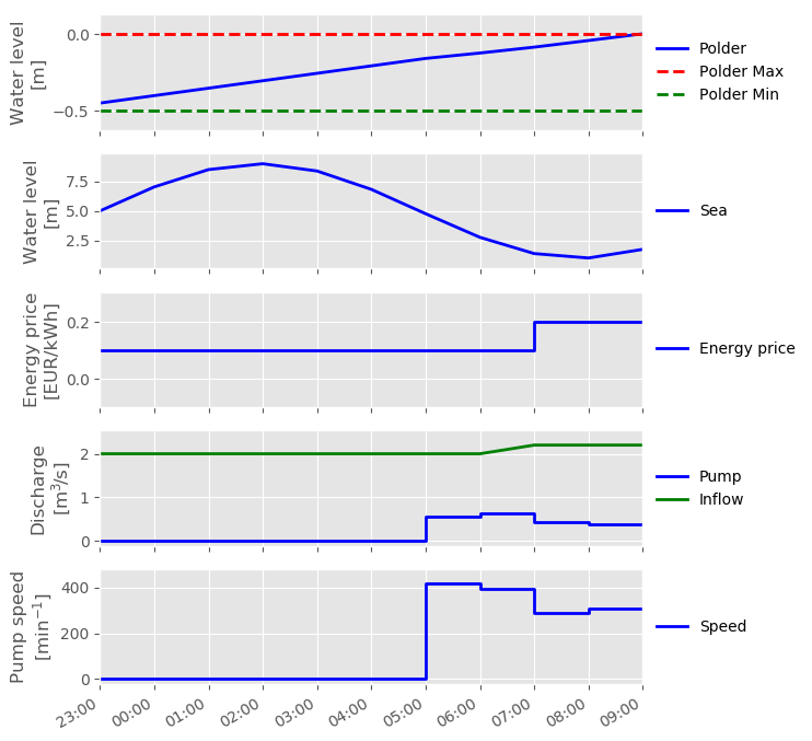
As expressed in the introduction of this example problem, we indeed see that the available buffer in the polder is used to its fullest. The water level at the final time step is (almost) equal to the maximum water level.
In this example, no historical data regarding the pump history is provided. Thus there is no prescribed behavior for the pump status on the initial time steps.
Furthermore, we see that the pump only discharges water when the water level is low. It is interesting to see that the optimal solution for costs means pumping at the lowest water level, even though the energy price is twice as high.
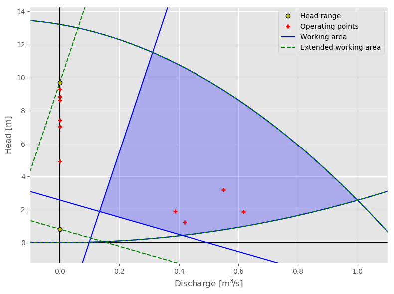
Using plot_operating_points()
it is possible to generate a Q-H plot of the pump’s working area and operating
points, such as shown below. Here we see that the pumping at lower heads
occurs with relatively large discharges, meaning that the pump is sometimes
operating close to the edges of its working area.