Constant speed pump

Note

This example focuses on how to model a constant speed pump, and assumes basic exposure to RTC-Tools and the PumpingStationMixin. To start with basics of pump modeling, see Basic Pumping Station.

The purpose of this example is to understand the technical setup of a model of a constant speed pump.

The scenario of this example is equal to that of Basic Pumping Station, but with one constant speed pump instead of a variable speed pump. The resistance has also been removed. The folder examples/pumping_station/two_pumps contains the complete RTC- Tools optimization problem. The discussion below will focus on the differences from the Basic Pumping Station.

Note

The resistance has been removed because it created an artificial head loss to be able to pump at lower power energy prices.

The Model

The constant speed pump is modeled the same way as the variable speed one. The difference is the working area and the power approximation. This can be seen in the file Example.mo:

    Deltares.HydraulicStructures.PumpingStation.Pump pump1(
      power_coefficients = {{{-39095.7484857 ,  66783.26438029},
                             {  7281.58399033,       0.0}},
                            {{-27859.72396609,  52991.89678362},
                             {  6547.78028277,       0.0}},
                            {{-23247.11759041,  47371.07046571},
                             {  6106.48287875,       0.0}},
                            {{-33451.06236192,  59110.131313  },
                             {  7034.0025483,       0.0}},
                            {{-39861.93265223,  67925.88638803},
                             {  7281.81109575,       0.0}},
                            {{-18905.97159263,  40725.7120928 },
                             {  5785.42670305,       0.0}},
                            {{-69080.26073112,  97844.92974535},
                             {  8776.27578528,       0.0}},
                            {{-27357.47031974,  52938.41395038},
                             {  6406.26137405,       0.0}},
                            {{-49670.43493511,  78653.65042992},
                             {  7840.68764271,       0.0}},

The interpretation and the calculation of these coefficients is explained in Modelica API. For constant speed pumps, the polynomial that defines the minimum and maximum speed is the same.

The Optimization Problem

The optimization problem is exactly the same as for a variable speed pump.

Results

The same example is calculated with a variable and a constant speed pump. The constant speed pump’s speed is equal to the maximum speed of the variable speed pump. The results with the variable speed pump

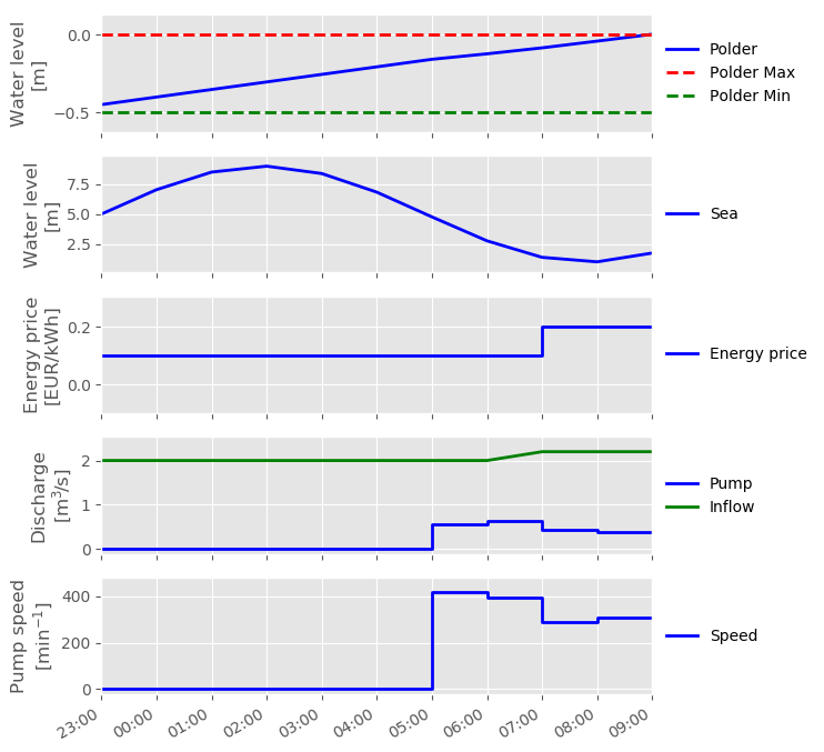
and the constant speed pump are shown below.

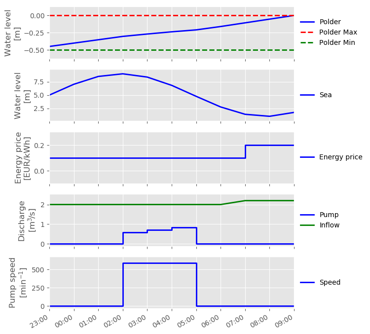
It can be seen that the constant speed pump was trying in a shorter time but pumping higher discharge. In this situation the constant speed pump therefore using three times more energy.

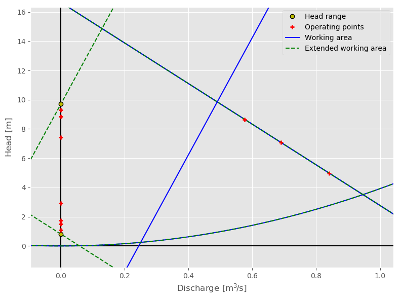
In the Q-H plot of the operating points we clearly see the pump operating on the linearized maximum pump speed line.