Basic Weir
Note
This example focuses on how to implement a controllable weir in RTC-Tools using the Hydraulic Structures library. It assumes basic exposure to RTC- Tools. If you are a first-time user of RTC-Tools, please refer to the RTC-Tools documentation.
The weir structure is valid for two flow conditions:
- Free (critical) flow
- No flow
Warning
Submerged flow is not supported.
Modeling
Building a model with a weir
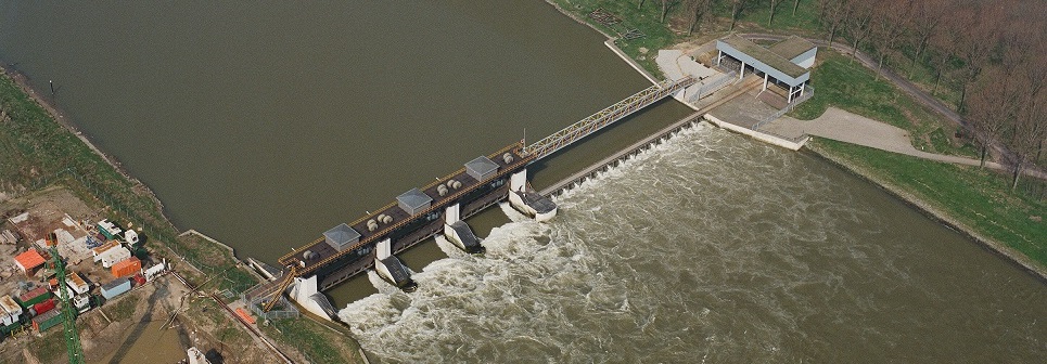
In this example we are considering a system of two branches and a controllable weir in between. On the upstream side is a prescribed input flow, and on the downstream side is a prescribed output flow. The weir should move in such way that the water level in both branches is kept within the desired limits.
- To build this model, we need the following blocks:
- upstream and downstream discharge boundary conditions
- two branches
- a weir
By putting the blocks from the Modelica editor, the code is automatically generated (Note: this code snippet excludes the lines about the annotation and location):
6 7 8 9 10 11 | output Modelica.SIunits.Volume branch_2_water_level;
Deltares.ChannelFlow.Hydraulic.BoundaryConditions.Discharge Upstream;
Deltares.ChannelFlow.Hydraulic.BoundaryConditions.Discharge Downstream;
Deltares.ChannelFlow.Hydraulic.Reservoir.Linear Branch1(A = 50, H_b = 0, H(nominal=1, min=0, max=100));
Deltares.ChannelFlow.Hydraulic.Reservoir.Linear Branch2(A = 100, H_b = 0, H(nominal=1, min=0, max=100));
Deltares.HydraulicStructures.Weir.Weir weir1(hw_max = 3, hw_min = 1.7, q_max = 1, q_min = 0, width = 10);
|
For the weir block, the dimensions of the weir should be set. It can be done either by double
clicking to the block, or in the text editor.
A controllable weir is represented with a weir block. This block has discharge and water level as input,
and also as output. When a block is placed, the following parameters can be given:
- width: the width of the crest in meters
- hw_min: the minimum crest height
- hw_max: the maximum crest height
- q_min: the minimum expected discharge
- q_max: the maximum expected discharge
The last two values should be estimated in such way that the discharge will not be able to go outside these bounds. However, for some linearization purposes, they should be as tight as possible. The values set by the text editor look like the line above.
The input variables are the upstream and downstream (known) discharges. The control variable - the variable that the algorithm changes until it achieves the desired results - is the discharge between the two branches. In practice, the weir height is the variable that we are interested in, but as it depends on the discharge between the two branches and the upstream water level, it will only be calculated in post processing. The input variables for the model are:
2 3 4 | input Modelica.SIunits.VolumeFlowRate upstream_q_ext(fixed = true);
input Modelica.SIunits.VolumeFlowRate downstream_q_ext(fixed = true);
input Modelica.SIunits.VolumeFlowRate WeirFlow1(fixed = false, nominal=1, min=0, max=2.5);
|
Important
The min, max and nominal the values should always be meaningful. For nominal, set the value that the variable most likely takes.
As output, we are interested in the water level in the two branches:
5 6 | output Modelica.SIunits.Volume branch_1_water_level;
output Modelica.SIunits.Volume branch_2_water_level;
|
Now we have to define the equations. We have to set the boundary conditions. First the discharge should be read from the external files:
21 22 | Upstream.Q = upstream_q_ext;
Downstream.Q = downstream_q_ext;
|
And then the water level should be defined equal to the water level in the branch:
17 18 | Branch1.HQDown.H=Branch1.H;
Branch2.HQDown.H=Branch2.H;
|
As we use reservoirs for branches, the variables we do not need should be zero:
19 20 | Branch1.Q_turbine=0;
Branch2.Q_turbine=0;
|
Finally the outputs are set:
24 25 | branch_1_water_level = Branch1.H;
branch_2_water_level = Branch2.H;
|
and the control variable as well:
23 | WeirFlow1 = weir1.Q;
|
The whole model file looks like this:
1 2 3 4 5 6 7 8 9 10 11 12 13 14 15 16 17 18 19 20 21 22 23 24 25 26 | model WeirExample
input Modelica.SIunits.VolumeFlowRate upstream_q_ext(fixed = true);
input Modelica.SIunits.VolumeFlowRate downstream_q_ext(fixed = true);
input Modelica.SIunits.VolumeFlowRate WeirFlow1(fixed = false, nominal=1, min=0, max=2.5);
output Modelica.SIunits.Volume branch_1_water_level;
  output Modelica.SIunits.Volume branch_2_water_level;
  Deltares.ChannelFlow.Hydraulic.BoundaryConditions.Discharge Upstream;
  Deltares.ChannelFlow.Hydraulic.BoundaryConditions.Discharge Downstream;
  Deltares.ChannelFlow.Hydraulic.Reservoir.Linear Branch1(A = 50, H_b = 0, H(nominal=1, min=0, max=100));
  Deltares.ChannelFlow.Hydraulic.Reservoir.Linear Branch2(A = 100, H_b = 0, H(nominal=1, min=0, max=100));
  Deltares.HydraulicStructures.Weir.Weir weir1(hw_max = 3, hw_min = 1.7, q_max = 1, q_min = 0, width = 10);
equation
connect(weir1.HQDown, Branch2.HQUp);
connect(Branch1.HQDown, weir1.HQUp);
connect(Branch2.HQDown, Downstream.HQ);
connect(Upstream.HQ, Branch1.HQUp);
Branch1.HQDown.H=Branch1.H;
Branch2.HQDown.H=Branch2.H;
Branch1.Q_turbine=0;
Branch2.Q_turbine=0;
  Upstream.Q = upstream_q_ext;
  Downstream.Q = downstream_q_ext;
WeirFlow1 = weir1.Q;
  branch_1_water_level = Branch1.H;
  branch_2_water_level = Branch2.H;
end WeirExample;
|
Optimization
In this example, we would like to achieve that the water levels in the branches stay in the prescribed
limits. The easiest way to achieve this objective is through goal programming. We will define two goals,
one goal for each branch. The goal is that the water level should be higher than the given minimum and
lower than the given maximum. Any solution satisfying these criteria is equally attractive for us.
In practice, in goal programming the goal violation value is taken to the order’th power in the objective function
(see: Goal Programming).
In our example, we use the file WeirExample.py. We define a class, and apart from the usual classes
that we import for optimization problems, we also have to import the class WeirMixin:
37 38 39 40 | class WeirExample(WeirMixin, GoalProgrammingMixin, CSVMixin, ModelicaMixin, CollocatedIntegratedOptimizationProblem):
def __init__(self, *args, **kwargs):
super(WeirExample, self).__init__(*args, **kwargs)
|
Now we have to define the weirs: in quotation marks should be the same name as used for the Modelica model. Now there is only one weir, and the definition looks like:
41 | self.__weirs = [Weir(self, 'weir1')]
|
In case of more weirs, the names can be separated with a comma, for example:
self._weirs = [Weir('weir1'), Weir('weir2')]
Lastly we have to override the abstract method the returns the list of weirs:
44 45 | def weirs(self):
return self.__weirs
|
Adding goals
In this example there are two branches connected with a weir. On the upstream side is a prescribed input flow, and on the downstream side is a prescribed output flow. The weir should move in such way, that the water level in both branches kept within the desired limits. We can add a water level goal for the upstream branch:
13 14 15 16 17 18 19 20 21 22 | class WLRangeGoal_01(StateGoal):
def __init__(self, optimization_problem):
self.state = 'Branch1.H'
self.priority = 1
self.target_min = optimization_problem.get_timeseries('h_min_branch1')
self.target_max = optimization_problem.get_timeseries('h_max_branch1')
super(WLRangeGoal_01, self).__init__(optimization_problem)
|
A similar goal can be added to the downstream branch.
Setting the solver
As it is a mixed integer problem, it is handy to set some options to control
the solver. In this example, we set the allowable_gap to 0.005. It is used
to specify the value of absolute gap under which the algorithm stops. This is
bigger than the default. This gives lower expectations for the acceptable
solution, and in this way, the time of iteration is less. This value might be
different for every problem and might be adjusted a trial-and-error basis. For
more information, see the documentation of the BONMIN solver User’s Manual)
The solver setting is the following:
47 48 49 50 51 | def solver_options(self):
options = super(WeirExample, self).solver_options()
options['allowable_gap'] = 0.005
options['print_level'] = 2
return options
|
Input data
In order to run the optimization, we need to give the boundary conditions and the water level bounds.
This data is given as time-series in the file timeseries_import.csv.
The whole python file
The optimization file looks like:
1 2 3 4 5 6 7 8 9 10 11 12 13 14 15 16 17 18 19 20 21 22 23 24 25 26 27 28 29 30 31 32 33 34 35 36 37 38 39 40 41 42 43 44 45 46 47 48 49 50 51 52 53 54 55 56 57 58 59 60 61 62 63 64 65 66 67 68 69 70 71 72 73 74 75 76 77 78 79 80 81 82 83 84 85 86 87 88 89 90 91 92 93 94 95 96 97 98 99 100 101 102 103 104 105 106 107 108 109 110 111 112 113 114 115 116 117 118 119 120 121 122 123 124 125 126 127 128 129 130 131 132 133 134 135 136 137 138 139 140 141 142 143 144 145 146 147 148 149 150 151 152 153 154 155 156 | from rtctools.optimization.collocated_integrated_optimization_problem \
import CollocatedIntegratedOptimizationProblem
from rtctools.optimization.goal_programming_mixin import GoalProgrammingMixin, StateGoal
from rtctools.optimization.modelica_mixin import ModelicaMixin
from rtctools.optimization.csv_mixin import CSVMixin
from rtctools.util import run_optimization_problem
from rtctools_hydraulic_structures.weir_mixin import WeirMixin, Weir, plot_operating_points
# There are two water level targets, with different priority.
# The water level should stay in the required range during all the simulation
class WLRangeGoal_01(StateGoal):
def __init__(self, optimization_problem):
self.state = 'Branch1.H'
self.priority = 1
self.target_min = optimization_problem.get_timeseries('h_min_branch1')
self.target_max = optimization_problem.get_timeseries('h_max_branch1')
super(WLRangeGoal_01, self).__init__(optimization_problem)
class WLRangeGoal_02(StateGoal):
def __init__(self, optimization_problem):
self.state = 'Branch2.H'
self.priority = 2
self.target_min = optimization_problem.get_timeseries('h_min_branch2')
self.target_max = optimization_problem.get_timeseries('h_max_branch2')
super(WLRangeGoal_02, self).__init__(optimization_problem)
class WeirExample(WeirMixin, GoalProgrammingMixin, CSVMixin, ModelicaMixin, CollocatedIntegratedOptimizationProblem):

    def __init__(self, *args, **kwargs):
        super(WeirExample, self).__init__(*args, **kwargs)
self.__weirs = [Weir(self, 'weir1')]
self.__output_folder = kwargs['output_folder'] # So we can write our pictures to it
    def weirs(self):
        return self.__weirs
    def solver_options(self):
        options = super(WeirExample, self).solver_options()
        options['allowable_gap'] = 0.005
        options['print_level'] = 2
        return options
def path_goals(self):
goals = super(WeirExample, self).path_goals()
goals.append(WLRangeGoal_01(self))
goals.append(WLRangeGoal_02(self))
return goals
def post(self):
super(WeirExample, self).post()
results = self.extract_results()
# Make plots
import matplotlib.dates as mdates
import matplotlib.pyplot as plt
import numpy as np
import os
plt.style.use('ggplot')
def unite_legends(axes):
h, l = [], []
for ax in axes:
tmp = ax.get_legend_handles_labels()
h.extend(tmp[0])
l.extend(tmp[1])
return h, l
# Plot #1: Data over time. X-axis is always time.
f, axarr = plt.subplots(4, sharex=True)
# TODO: Do not use private API of CSVMixin
times = self._timeseries_times
weir = self.weirs()[0]
axarr[0].set_ylabel('Water level\n[m]')
axarr[0].plot(times, results['branch_1_water_level'], label='Upstream',
linewidth=2, color='b')
axarr[0].plot(times, self.get_timeseries('h_min_branch1').values, label='Upstream Max',
linewidth=2, color='r', linestyle='--')
axarr[0].plot(times, self.get_timeseries('h_max_branch1').values, label='Upstream Min',
linewidth=2, color='g', linestyle='--')
ymin, ymax = axarr[0].get_ylim()
axarr[0].set_ylim(ymin - 0.1, ymax + 0.1)
axarr[1].set_ylabel('Water level\n[m]')
axarr[1].plot(times, results['branch_2_water_level'], label='Downstream',
linewidth=2, color='b')
axarr[1].plot(times, self.get_timeseries('h_max_branch2').values, label='Downstream Max',
linewidth=2, color='r', linestyle='--')
axarr[1].plot(times, self.get_timeseries('h_min_branch2').values, label='Downstream Min',
linewidth=2, color='g', linestyle='--')
ymin, ymax = axarr[1].get_ylim()
axarr[1].set_ylim(ymin - 0.1, ymax + 0.1)
axarr[2].set_ylabel('Discharge\n[$\mathdefault{m^3\!/s}$]')
# We need the first point for plotting, but its value does not
# necessarily make sense as it is not included in the optimization.
weir_flow = results['WeirFlow1']
weir_height = results["weir1_height"]
minimum_water_level_above_weir = (weir_flow-weir.q_nom)/weir.slope + weir.h_nom
minimum_weir_height = minimum_water_level_above_weir - ((weir_flow/weir.c_weir)**(2.0/3.0))
minimum_weir_height[0] = minimum_weir_height[1]
weir_flow = results['WeirFlow1']
weir_flow[0] = weir_flow[1]
axarr[2].step(times, weir_flow, label='Weir',
linewidth=2, color='b')
axarr[2].step(times, self.get_timeseries('upstream_q_ext').values, label='Inflow',
linewidth=2, color='r', linestyle='--')
axarr[2].step(times, -1 * self.get_timeseries('downstream_q_ext').values, label='Outflow',
linewidth=2, color='g', linestyle='--')
ymin, ymax = axarr[2].get_ylim()
axarr[2].set_ylim(-0.1, ymax + 0.1)
weir_height = results["weir1_height"]
weir_height[0] = weir_height[1]
axarr[3].set_ylabel('Weir height\n[m]')
axarr[3].step(times, weir_height, label='Weir',
linewidth=2, color='b')
ymin, ymax = axarr[3].get_ylim()
ymargin = 0.1 * (ymax - ymin)
axarr[3].set_ylim(ymin - ymargin, ymax + ymargin)
axarr[3].xaxis.set_major_formatter(mdates.DateFormatter('%H:%M'))
f.autofmt_xdate()
# Shrink each axis by 20% and put a legend to the right of the axis
for i in range(len(axarr)):
box = axarr[i].get_position()
axarr[i].set_position([box.x0, box.y0, box.width * 0.8, box.height])
axarr[i].legend(loc='center left', bbox_to_anchor=(1, 0.5), frameon=False)
# Output Plot
f.set_size_inches(8, 9)
plt.savefig(os.path.join(self.__output_folder, 'overall_results.png'),
bbox_inches='tight', pad_inches=0.1)
plot_operating_points(self, self._output_folder, results)
if __name__ == "__main__":
run_optimization_problem(WeirExample)
|
Results
After successful optimization the results are printed in the time series export file. After running this example, the following results are expected:
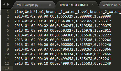
The file found in the example folder includes some visualization routines.
Interpretation of the results
The results of this simulation are summarized in the following figure:
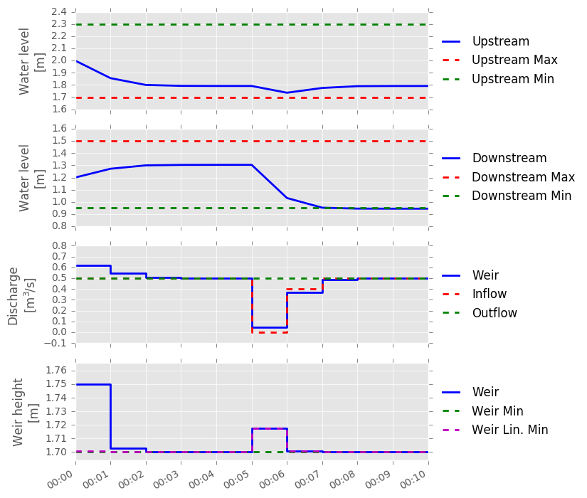
In this example, the input flow increases after 6 minutes, while the downstream flow is kept constant. While the inflow drops after 6 minutes, the result is not seen in the upstream branch, because the weir moves up to compensate it. After the weir moved up, the water level drops in the downstream branch.